Levi-Civita symbol

Not to be confused with Levi-Civita connection.

The Levi-Civita symbol, also called the permutation symbol, antisymmetric symbol, or alternating symbol, is a mathematical symbol used in particular in tensor calculus. It is named after the Italian mathematician and physicist Tullio Levi-Civita.

1 Definition
- 1.1 Relation to Kronecker delta
- 1.2 Generalization to n dimensions
2 Properties
- 2.1 Proofs
3 Examples
4 Notation
5 Tensor density
- 5.1 Ordinary tensor
6 See also
7 References

Definition

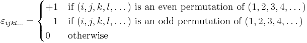
In three dimensions, the Levi-Civita symbol is defined as follows:

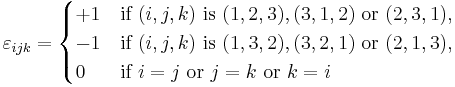
$\varepsilon_{ijk} = \begin{cases} %2B1 & \mbox{if } (i,j,k) \mbox{ is } (1,2,3), (3,1,2) \mbox{ or } (2,3,1), \\ -1 & \mbox{if } (i,j,k) \mbox{ is } (1,3,2), (3,2,1) \mbox{ or } (2,1,3), \\ 0 & \mbox{if }i=j \mbox{ or } j=k \mbox{ or } k=i \end{cases}$

i.e. $\varepsilon_{ijk}$ is 1 if (i, j, k) is an even permutation of (1,2,3), −1 if it is an odd permutation, and 0 if any index is repeated.

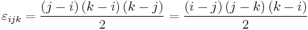
The formula for the three dimensional Levi-Civita symbol is:

$\varepsilon_{ijk} = \frac{\left( j-i \right)\left( k-i \right)\left( k-j \right)}{2} = \frac{\left( i-j \right)\left( j-k \right)\left( k-i \right)}{2}$

The formula in four dimensions is:

$\varepsilon_{ijkl} = \frac{\left( j-i \right)\left( k-i \right)\left( l-i \right)\left( k-j \right)\left( l-j \right)\left( l-k \right)}{12} = \frac{\left( i-j \right)\left( i-k \right)\left( i-l \right)\left( j-k \right)\left( j-l \right)\left( k-l \right)}{12}$

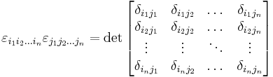
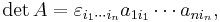
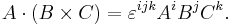
For example, in linear algebra, the determinant of a 3×3 matrix A can be written

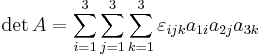
$\det A = \sum_{i=1}^3 \sum_{j=1}^3 \sum_{k=1}^3 \varepsilon_{ijk} a_{1i} a_{2j} a_{3k}$

(and similarly for a square matrix of general size, see below)

and the cross product of two vectors can be written as a determinant:

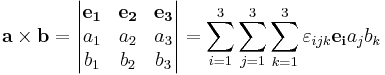
$\mathbf{a \times b} = \begin{vmatrix} \mathbf{e_1} & \mathbf{e_2} & \mathbf{e_3} \\ a_1 & a_2 & a_3 \\ b_1 & b_2 & b_3 \\ \end{vmatrix} = \sum_{i=1}^3 \sum_{j=1}^3 \sum_{k=1}^3 \varepsilon_{ijk} \mathbf{e_i} a_j b_k$

or more simply:

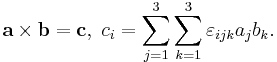
$\mathbf{a \times b} = \mathbf{c},\ c_i = \sum_{j=1}^3 \sum_{k=1}^3 \varepsilon_{ijk} a_j b_k.$

According to the Einstein notation, the summation symbols may be omitted.

The tensor whose components in an orthonormal basis are given by the Levi-Civita symbol (a tensor of covariant rank n) is sometimes called the permutation tensor. It is actually a pseudotensor because under an orthogonal transformation of jacobian determinant −1 (i.e., a rotation composed with a reflection), it acquires a minus sign. Because the Levi-Civita symbol is a pseudotensor, the result of taking a cross product is a pseudovector, not a vector.

Note that under a general coordinate change, the components of the permutation tensor get multiplied by the jacobian of the transformation matrix. This implies that in coordinate frames different from the one in which the tensor was defined, its components can differ from those of the Levi-Civita symbol by an overall factor. If the frame is orthonormal, the factor will be ±1 depending on whether the orientation of the frame is the same or not.

Relation to Kronecker delta

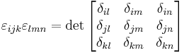
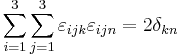
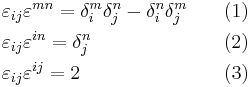
The Levi-Civita symbol is related to the Kronecker delta. In three dimensions, the relationship is given by the following equations:

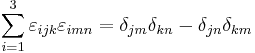$\varepsilon_{ijk}\varepsilon_{lmn} = \det \begin{bmatrix} \delta_{il} & \delta_{im}& \delta_{in}\\ \delta_{jl} & \delta_{jm}& \delta_{jn}\\ \delta_{kl} & \delta_{km}& \delta_{kn}\\ \end{bmatrix}$

$= \delta_{il}\left( \delta_{jm}\delta_{kn} - \delta_{jn}\delta_{km}\right) - \delta_{im}\left( \delta_{jl}\delta_{kn} - \delta_{jn}\delta_{kl} \right) %2B \delta_{in} \left( \delta_{jl}\delta_{km} - \delta_{jm}\delta_{kl} \right) \,$

$\sum_{i=1}^3 \varepsilon_{ijk}\varepsilon_{imn} = \delta_{jm}\delta_{kn} - \delta_{jn}\delta_{km}$ ("contracted epsilon identity")

In Einstein notation, the duplication of the i index implies the sum on i. The previous is then denoted: $\varepsilon_{ijk}\varepsilon_{imn} = \delta_{jm}\delta_{kn} - \delta_{jn}\delta_{km}\,.$

$\sum_{i=1}^3 \sum_{j=1}^3 \varepsilon_{ijk}\varepsilon_{ijn} = 2\delta_{kn}$

Generalization to n dimensions

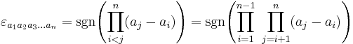
The Levi-Civita symbol can be generalized to higher dimensions:

$\varepsilon_{ijkl\dots} = \begin{cases} %2B1 & \mbox{if }(i,j,k,l,\dots) \mbox{ is an even permutation of } (1,2,3,4,\dots) \\ -1 & \mbox{if }(i,j,k,l,\dots) \mbox{ is an odd permutation of } (1,2,3,4,\dots) \\ 0 & \mbox{otherwise} \end{cases}$

Thus, it is the sign of the permutation in the case of a permutation, and zero otherwise.

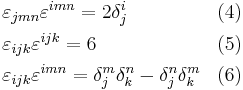
Some generalized formulae are:

$\varepsilon_{a_1 a_2 a_3 \ldots a_n} = \sgn \! \left( \prod_{i<j}^n ( a_j-a_i ) \right) = \sgn \! \left( \prod_{i=1}^{n-1} \ \prod_{j=i%2B1}^n ( a_j-a_i ) \right)$

where n is the dimension (rank), and

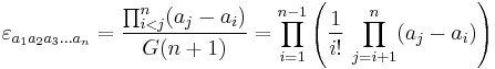
$\varepsilon_{a_1 a_2 a_3 \ldots a_n} = \frac{\prod_{i<j}^n ( a_j-a_i )}{G(n%2B1)} = \prod_{i=1}^{n-1} \left( \frac{1}{i!} \, \prod_{j=i%2B1}^n ( a_j-a_i ) \right)$

where G(n) is the Barnes G-function.

For any n, the property

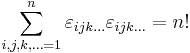
$\sum_{i,j,k,\dots=1}^n \varepsilon_{ijk\dots}\varepsilon_{ijk\dots} = n!$

follows from the facts that (a) every permutation is either even or odd, (b) (+1)² = (-1)² = 1, and (c) the permutations of any n-element set number exactly n!.

In index-free tensor notation, the Levi-Civita symbol is replaced by the concept of the Hodge dual.

In general, for n dimensions, one can write the product of two Levi-Civita symbols as:

$\varepsilon_{i_1 i_2 \dots i_n} \varepsilon_{j_1 j_2 \dots j_n} = \det \begin{bmatrix} \delta_{i_1 j_1} & \delta_{i_1 j_2} & \dots & \delta_{i_1 j_n} \\ \delta_{i_2 j_1} & \delta_{i_2 j_2} & \dots & \delta_{i_2 j_n} \\ \vdots & \vdots & \ddots & \vdots \\ \delta_{i_n j_1} & \delta_{i_n j_2} & \dots & \delta_{i_n j_n} \\ \end{bmatrix}$ .

Properties

(in these examples, superscripts should be considered equivalent with subscripts)

1. In two dimensions, when all $i,j,m,n$ are in $\{1,2\}$ ,

$\begin{align}&\varepsilon_{ij} \varepsilon^{mn} = \delta^m_i \delta^n_j - \delta^n_i \delta^m_j \quad &&(1) \\&\varepsilon_{ij} \varepsilon^{in} = \delta^n_j &&(2) \\&\varepsilon_{ij} \varepsilon^{ij} = 2 &&(3)\end{align}$

2. In three dimensions, when all $i,j,k,m,n$ are in $\{1,2,3\},$

$\begin{align}&\varepsilon_{jmn} \varepsilon^{imn}=2\delta^i_j &&(4)\\&\varepsilon_{ijk} \varepsilon^{ijk}=6 &&(5)\\&\varepsilon_{ijk} \varepsilon^{imn}=\delta^{m}_j\delta^{n}_k - \delta^{n}_j\delta^{m}_k &&(6)\end{align}$

3. In n dimensions, when all 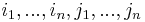$i_1,...,i_n,j_1,...,j_n$ are in $\{1,...,n\},$ :

$\begin{align}& \varepsilon_{i_1 \dots i_n} \varepsilon^{j_1 \dots j_n} = n! \delta^{j_1}_{[ i_1} \dots \delta^{j_n}_{i_n ]} &&(7)\\& \varepsilon_{i_1 \dots i_k~i_{k%2B1}\dots i_n} \varepsilon^{i_1 \dots i_k~j_{k%2B1}\dots j_n}= k!(n-k)!~\delta^{j_{k%2B1}}_{[ i_{k%2B1}} \dots \delta^{j_n}_{i_n ]} &&(8)\\& \varepsilon_{i_1 \dots i_n}\varepsilon^{i_1 \dots i_n} = n! &&(9)\end{align}$

Proofs

For equation 1, both sides are antisymmetric with respect of $ij$ and $mn$ . We therefore only need to consider the case $i\neq j$ and $m\neq n$ . By substitution, we see that the equation holds for $\varepsilon_{12} \varepsilon^{12}$ , i.e., for $i=m=1$ and $j=n=2$ . (Both sides are then one). Since the equation is antisymmetric in $ij$ and $mn$ , any set of values for these can be reduced to the above case (which holds). The equation thus holds for all values of $ij$ and $mn$ . Using equation 1, we have for equation 2 $\varepsilon_{ij}\varepsilon^{in}$ $=$ $\delta_i^i \delta_j^n - \delta^n_i \delta^i_j$

$=$ $2 \delta_j^n - \delta^n_j$

$=$ $\delta_j^n$ .

Here we used the Einstein summation convention with $i$ going from $1$ to $2$ . Equation 3 follows similarly from equation 2. To establish equation 4, let us first observe that both sides vanish when $i\neq j$ . Indeed, if $i\neq j$ , then one can not choose $m$ and $n$ such that both permutation symbols on the left are nonzero. Then, with $i=j$ fixed, there are only two ways to choose $m$ and $n$ from the remaining two indices. For any such indices, we have 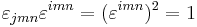$\varepsilon_{jmn} \varepsilon^{imn} = (\varepsilon^{imn})^2 = 1$ (no summation), and the result follows. Property (5) follows since $3!=6$ and for any distinct indices $i,j,k$ in $\{1,2,3\}$ , we have $\varepsilon_{ijk} \varepsilon^{ijk}=1$ (no summation).

Examples

1. The determinant of an $n\times n$ matrix $A=(a_{ij})$ can be written as

$\det A = \varepsilon_{i_1\cdots i_n} a_{1i_1} \cdots a_{ni_n},$

where each $i_l$ should be summed over $1,\ldots, n.$

Equivalently, it may be written as

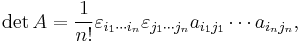
$\det A = \frac{1}{n!} \varepsilon_{i_1\cdots i_n} \varepsilon_{j_1\cdots j_n} a_{i_1 j_1} \cdots a_{i_n j_n},$

where now each $i_l$ and each $j_l$ should be summed over $1,\ldots, n$ .

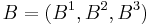2. If $A=(A^1, A^2, A^3)$ and $B=(B^1, B^2, B^3)$ are vectors in $R^3$ (represented in some right hand oriented orthonormal basis), then the $i$ th component of their cross product equals

$(A\times B)^i = \varepsilon^{ijk} A^j B^k.$

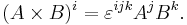
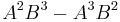For instance, the first component of $A\times B$ is $A^2 B^3-A^3 B^2$ . From the above expression for the cross product, it is clear that 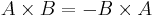$A\times B = -B\times A$ . Further, if 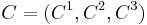$C=(C^1, C^2, C^3)$ is a vector like $A$ and $B$ , then the triple scalar product equals

$A\cdot(B\times C) = \varepsilon^{ijk} A^i B^j C^k.$

From this expression, it can be seen that the triple scalar product is antisymmetric when exchanging any adjacent arguments. For example, $A\cdot(B\times C)= -B\cdot(A\times C)$ .

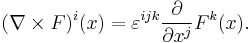
3. Suppose 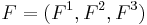$F=(F^1, F^2, F^3)$ is a vector field defined on some open set of $R^3$ with Cartesian coordinates 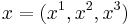$x=(x^1, x^2, x^3)$ . Then the $i$ th component of the curl of $F$ equals

$(\nabla \times F)^i(x) = \varepsilon^{ijk}\frac{\partial}{\partial x^j} F^k(x).$

Notation

Main article: Antisymmetric tensor

A shorthand notation for anti-symmetrization is denoted by a pair of square brackets. For example, in arbitrary dimensions, for a rank 2 covariant tensor M,

$M_{[ab]} = \frac{1}{2!}(M_{ab} - M_{ba}) \,,$

and for a rank 3 covariant tensor T,

$T_{[abc]} = \frac{1}{3!}(T_{abc}-T_{acb}%2BT_{bca}-T_{bac}%2BT_{cab}-T_{cba}) \,.$

In three dimensions, these are equivalent to

$M_{[ab]} = \varepsilon_{abc} \, \frac{1}{2!} \, \varepsilon^{dec} M_{de} \,,$

$T_{[abc]} = \varepsilon_{abc} \, \frac{1}{3!} \, \varepsilon^{def} T_{def} \,.$

While in four dimensions, these are equivalent to

$M_{[ab]} = \frac{1}{2!} \, \varepsilon_{abcd} \, \frac{1}{2!} \, \varepsilon^{efcd} M_{ef} \,,$

$T_{[abc]} = \varepsilon_{abcd} \, \frac{1}{3!} \, \varepsilon^{efgd} T_{efg} \,.$

More generally, in n dimensions

$S_{[a_1 \dots a_i]} = \frac{1}{(n-i)!} \varepsilon_{a_1 \dots a_i~b_1 \dots b_{n-i}} \frac{1}{i!} \varepsilon^{c_1 \dots c_i~b_1 \dots b_{n-i}} S_{c_1 \dots c_i} \,.$

Tensor density

In any arbitrary curvilinear coordinate system and even in the absence of a metric on the manifold, the Levi-Civita symbol as defined above may be considered to be a tensor density field in two different ways. It may be regarded as a contravariant tensor density of weight +1 or as a covariant tensor density of weight -1. In four dimensions,

$\varepsilon^{\alpha \beta \gamma \delta} = \varepsilon_{\alpha \beta \gamma \delta} \,.$

Notice that the value, and in particular the sign, does not change.

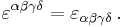
Ordinary tensor

In the presence of a metric tensor field, one may define an ordinary contravariant tensor field which agrees with the Levi-Civita symbol at each event whenever the coordinate system is such that the metric is orthonormal at that event. Similarly, one may also define an ordinary covariant tensor field which agrees with the Levi-Civita symbol at each event whenever the coordinate system is such that the metric is orthonormal at that event. These ordinary tensor fields should not be confused with each other, nor should they be confused with the tensor density fields mentioned above. One of these ordinary tensor fields may be converted to the other by raising or lowering the indices with the metric as is usual, but a minus sign is needed if the metric signature contains an odd number of negatives. For example, in Minkowski space (the four dimensional spacetime of special relativity)

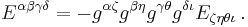
$E^{\alpha \beta \gamma \delta} = - g^{\alpha \zeta} g^{\beta \eta} g^{\gamma \theta} g^{\delta \iota} E_{\zeta \eta \theta \iota} \,.$

Notice the minus sign.

References

Charles W. Misner, Kip S. Thorne, John Archibald Wheeler, Gravitation, (1970) W.H. Freeman, New York; ISBN 0-7167-0344-0. (See section 3.5 for a review of tensors in general relativity).

This article incorporates material from Levi-Civita permutation symbol on PlanetMath, which is licensed under the Creative Commons Attribution/Share-Alike License.